In this paper a generalized Akash distribution (GAD) which includes Akash distribution of Shanker¹ and exponential distribution as particular cases has been introduced and studied. Its mathematical and statistical properties including its shapes for varying values of parameters, moments based measures, hazard rate function, mean residual life function, stochastic ordering, mean deviations, order statistics, Renyi entropy measure, Bonferroni and Lorenz curves and stress-strength reliability has been studied. The estimation of its parameters has been discussed using both the method of moments and the maximum likelihood estimation. Goodness of fit of GAD has been explained through a real lifetime data and the fit has been compared with other lifetime distributions.

Keywords: akash distribution, moments and associated measures, reliability measures, stochastic ordering, order statistics, renyi entropy measure, mean deviations, bonferroni and lorenz curves, estimation of parameters, goodness of fit

Shanker¹ introduced a one-parameter lifetime distribution, known as Akash distribution, defined by its probability density function (pdf) and cumulative distribution function (cdf)

$f_1\left(x;\theta \right)=\frac{{\theta }^3}{{\theta }^2+2}\left(1+x^2\right)e^{-\theta x};x>0,\theta >0$   (1.1)

$F_1\left(x;\theta \right)=1-\left[1+\frac{\theta x\left(\theta x+2\right)}{{\theta }^2+2}\right]e^{-\theta x};x>0,\theta >0$   (1.2)

This distribution is a two-component mixture of exponential $\left(\theta \right)$ and gamma $\left(3,\theta \right)$ distributions with their mixing proportions $\frac{{\theta }^2}{{\theta }^2+2}$ and $\frac{1}{{\theta }^2+2}$ respectively. Shanker¹ has discussed its various mathematical and statistical properties and showed that in many ways (1.1) provides a better model for modeling lifetime data from medical science and engineering than Lindley² and exponential distributions. Shanker et al.^3,4 have detailed comparative and critical study on Akash, Lindley and exponential distributions for modeling lifetime data from biomedical science and engineering and observed that Akash distribution provides better fit than both Lindley and exponential distributions in almost all lifetime datasets.

The first four moments about origin of Akash distribution obtained by Shanker¹ are given by

${{\mu }_1}^{\text{'}}=\frac{{\theta }^2+6}{\theta \left({\theta }^2+2\right)},{{\mu }_2}^{\text{'}}=\frac{2\left({\theta }^2+12\right)}{{\theta }^2\left({\theta }^2+2\right)},{{\mu }_3}^{\text{'}}=\frac{6\left({\theta }^2+20\right)}{{\theta }^3\left({\theta }^2+2\right)},{{\mu }_4}^{\text{'}}=\frac{24\left({\theta }^2+30\right)}{{\theta }^4\left({\theta }^2+2\right)}$

The central moments of Akash distribution as obtained by Shanker¹ are

${\mu }_2=\frac{{\theta }^4+16{\theta }^2+12}{{\theta }^2{\left({\theta }^2+2\right)}^2}$

${\mu }_3=\frac{2\left({\theta }^6+30{\theta }^4+36{\theta }^2+24\right)}{{\theta }^3{\left({\theta }^2+2\right)}^3}$

${\mu }_4=\frac{3\left(3{\theta }^8+128{\theta }^6+408{\theta }^4+576{\theta }^2+240\right)}{{\theta }^4{\left({\theta }^2+2\right)}^4}$

Shanker⁵ obtained Poisson- Akash distribution (PAD), a Poisson mixture of Akash distribution, and discussed its various statistical and mathematical properties along with estimation of parameter and applications for counts data from different fields of knowledge. Shanker^6,7 has also introduced size-biased and zero-truncated version of PAD and studied their statistical properties, estimation of parameter and applications for count datasets which structurally excludes zero counts.

In this paper, a generalized Akash distribution (GAD), of which the Akash distribution (1.1) of Shanker¹ and exponential distribution are special cases, has been suggested. Its shapes for varying values of parameters, moments and moments based properties have been derived and discussed. The hazard rate function, mean residual life function, stochastic ordering, mean deviations, order statistics, Renyi entropy measure, Bonferroni and Lorenz curves, and stress-strength reliability of GAD have been derived and discussed. The estimation of parameters has been discussed using both the method of moments and the maximum likelihood estimation. Finally, goodness of fit of GAD has been discussed with a real lifetime dataset and the fit has been compared with some well known distributions.

 A two-parameter generalized Akash distribution (GAD) with parameters  $\theta$ and $\alpha$ is defined by its pdf

$f_2\left(x;\theta ,\alpha \right)=\frac{{\theta }^3}{{\theta }^2+2\alpha }\left(1+\alpha x^2\right)e^{-\theta x};x>0,\theta >0,\alpha >0$   (2.1)

It can be easily verified that the Akash distribution defined in (1.1) and exponential distribution are particular cases of GAD (2.1) at $\alpha =1$ and $\alpha =0$ respectively. The pdf (2.1) can be shown as a two-component mixture of exponential $\left(\theta \right)$ and gamma $\left(3,\theta \right)$ distributions. We have

$f_2\left(x;\theta ,\alpha \right)=p{g}_1\left(x,\theta \right)+\left(1-p\right)g_2\left(x;3,\theta \right)$   (2.2)

where $p=\frac{{\theta }^2}{{\theta }^2+2\alpha },g_1\left(x,\theta \right)=\theta e^{-\theta x}$ and $g_2\left(x\right)=\frac{{\theta }^3}{\Gamma \left(3\right)}{e}^{-\theta x}{x}^{3-1}$

The corresponding cdf of GAD (2.1) can be obtained as          

$F_2\left(x;\theta ,\alpha \right)=1-\left[1+\frac{\alpha \theta x\left(\theta x+2\right)}{{\theta }^2+2\alpha }\right]e^{-\theta x};x>0,\theta >0,\alpha >0$   (2.3)

The graphs of pdf and cdf of GAD for varying values of parameters are shown in figures 1 and 2.

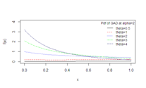
Figure 1 pdf of GAD for varying values of parameters $\theta$ and $\alpha$.

Figure 2 cdf of GAD for varying values of parameters $\theta$ and $\alpha$.

The moment generating function (mgf) about origin of GAD (2.1) can be obtained as

$M_X\left(t\right)=\frac{{\theta }^3}{{\theta }^2+2\alpha }\underset{0}{\overset{\infty }{\int }}{e}^{-\left(\theta -t\right)x}\left(1+\alpha x^2\right)dx$

$=\frac{{\theta }^3}{{\theta }^2+2\alpha }\left[\frac{1}{\left(\theta -t\right)}+\frac{2\alpha }{{\left(\theta -t\right)}^3}\right]$

$=\frac{{\theta }^3}{{\theta }^2+2\alpha }\left[\frac{1}{\theta }\sum _{k=0}^{\infty }{\left(\frac{t}{\theta }\right)}^k+\frac{2\alpha }{{\theta }^3}\sum _{k=0}^{\infty }\left(\begin{array}{c}k+2\\ k\end{array}\right){\left(\frac{t}{\theta }\right)}^k\right]$

$=\sum _{k=0}^{\infty }\frac{{\theta }^2+\left(k+1\right)\left(k+2\right)\alpha }{{\theta }^2+2\alpha }{\left(\frac{t}{\theta }\right)}^k$

The rth moment about origin of GAD (2.1) thus can be obtained as

${{\mu }_r}^{\text{'}}=\frac{r!\left\{{\theta }^2+\left(r+1\right)\left(r+2\right)\alpha \right\}}{{\theta }^r\left({\theta }^2+2\alpha \right)};r=1,2,3,\mathrm{...}$   (3.1)

Taking $r=1,2,3$ and 4 in (3.1), the first four moments about origin of GAD (2.1) are obtained as

${{\mu }_1}^{\text{'}}=\frac{{\theta }^2+6\alpha }{\theta \left({\theta }^2+2\alpha \right)},{{\mu }_2}^{\text{'}}=\frac{2\left({\theta }^2+12\alpha \right)}{{\theta }^2\left({\theta }^2+2\alpha \right)},{{\mu }_3}^{\text{'}}=\frac{6\left({\theta }^2+20\alpha \right)}{{\theta }^3\left({\theta }^2+2\alpha \right)},{{\mu }_4}^{\text{'}}=\frac{24\left({\theta }^2+30\alpha \right)}{{\theta }^4\left({\theta }^2+2\alpha \right)}$

Using the relationship between moments about origin and central moments, central moments of GAD (2.1) are obtained as

${\mu }_2=\frac{{\theta }^4+16{\theta }^2\alpha +12{\alpha }^2}{{\theta }^2{\left({\theta }^2+2\alpha \right)}^2}$

${\mu }_3=\frac{2\left({\theta }^6+30{\theta }^4\alpha +36{\theta }^2{\alpha }^2+24{\alpha }^3\right)}{{\theta }^3{\left({\theta }^2+2\alpha \right)}^3}$

${\mu }_4=\frac{3\left(3{\theta }^8+128{\theta }^6\alpha +408{\theta }^4{\alpha }^2+576{\theta }^2{\alpha }^3+240{\alpha }^4\right)}{{\theta }^4{\left({\theta }^2+2\alpha \right)}^4}$

The coefficients of variation $\left(\gamma \right)$ , skewness $\left(\sqrt{{\beta }_1}\right)$, kurtosis $\left({\beta }_2\right)$ and index of dispersion $\left(\gamma \right)$ of GAD are thus obtained as

$C.V=\frac{\sigma }{{{\mu }_1}^{\text{'}}}=\frac{\sqrt{{\theta }^4+16{\theta }^2\alpha +12{\alpha }^2}}{{\theta }^2+6\alpha }$

$\sqrt{{\beta }_1}=\frac{{\mu }_3}{{{\mu }_2}^{3/2}}=\frac{2\left({\theta }^6+30{\theta }^4\alpha +36{\theta }^2{\alpha }^2+24{\alpha }^3\right)}{{\left({\theta }^4+16{\theta }^2\alpha +12{\alpha }^2\right)}^{3/2}}$

${\beta }_2=\frac{{\mu }_4}{{{\mu }_2}^2}=\frac{3\left(3{\theta }^8+128{\theta }^6\alpha +408{\theta }^4{\alpha }^2+576{\theta }^2{\alpha }^3+240{\alpha }^4\right)}{{\left({\theta }^4+16{\theta }^2\alpha +12{\alpha }^2\right)}^2}$

$\gamma =\frac{{\sigma }^2}{{{\mu }_1}^{\text{'}}}\text{= }\frac{{\theta }^4+16{\theta }^2\alpha +12{\alpha }^2}{\theta \left({\theta }^2+2\alpha \right)\left({\theta }^2+6\alpha \right)}$

It can be easily verified that these statistical constants of GAD reduces to the corresponding statistical constants of Akash and exponential distributions at $\alpha =1$ and $\alpha =0$ respectively. Graphs of coefficient of variation, coefficient of skewness, coefficient of kurtosis and index of dispersion of GAD for varying values of parameters and have been drawn and presented in Figure 3.

Figure 3 Graphs of coefficient of variation, coefficient of skewness, coefficient of kurtosis and index of dispersion of GAD for varying values of parameters $\theta$ and $\alpha$.

Stochastic ordering

Stochastic ordering of positive continuous random variables is an important tool for judging the comparative behavior. A random variable $X$ is said to be smaller than a random variable $Y$ in the

1. stochastic order $\left(X{\le }_{st}Y\right)$ if $F_X\left(x\right)\ge F_Y\left(x\right)$ for all $x$
2. hazard rate order $\left(X{\le }_{hr}Y\right)$ if $h_X\left(x\right)\ge h_Y\left(x\right)$ for all $x$
3. mean residual life order $\left(X{\le }_{mrl}Y\right)$ if $m_X\left(x\right)\le m_Y\left(x\right)$ for all $x$
4. likelihood ratio order $\left(X{\le }_{lr}Y\right)$ if $\frac{f_X\left(x\right)}{f_Y\left(x\right)}$ decreases in$x$.

The following results due to Shaked and Shanthikumar⁸ are well known for establishing stochastic ordering of distributions

$\begin{array}{l}X{\le }_{lr}Y\Rightarrow X{\le }_{hr}Y\Rightarrow X{\le }_{mrl}Y\\ \underset{X{\le }_{st}Y}{\Downarrow }\end{array}$

The GAD is ordered with respect to the strongest "likelihood ratio" ordering as established in the following theorem:

Theorem: Let $X$$~$ GAD $\left({\theta }_1,{\alpha }_1\right)$  and $Y~GAD \left({\theta }_2,{\alpha }_2\right)$. If ${\alpha }_1={\alpha }_2$ and ${\theta }_1\ge {\theta }_2$(or if ${\theta }_1={\theta }_2$ and ${\alpha }_1\le {\alpha }_2$), then $X{\le }_{lr}Y$ and hence $X{\le }_{hr}Y$, $X{\le }_{mrl}Y$ and $X{\le }_{st}Y$.

P roof: We have

$\frac{f_X\left(x;{\theta }_1,{\alpha }_1\right)}{f_Y\left(x;{\theta }_2,{\alpha }_2\right)}=\frac{{{\theta }_1}^3\left({{\theta }_2}^2+2{\alpha }_2\right)}{{{\theta }_2}^3\left({{\theta }_1}^2+2{\alpha }_1\right)}\left(\frac{1+{\alpha }_1{x}^2}{1+{\alpha }_2{x}^2}\right)e^{-\left({\theta }_1-{\theta }_2\right)x};x>0$

Now

$\ln \frac{f_X\left(x;{\theta }_1,{\alpha }_1\right)}{f_Y\left(x;{\theta }_2,{\alpha }_2\right)}=\ln \left[\frac{{{\theta }_1}^3\left({{\theta }_2}^2+2{\alpha }_2\right)}{{{\theta }_2}^3\left({{\theta }_1}^2+2{\alpha }_1\right)}\right]+\ln \left(\frac{1+{\alpha }_1{x}^2}{1+{\alpha }_2{x}^2}\right)-\left({\theta }_1-{\theta }_2\right)x$ .

Thus

$\frac{d}{dx}\left\{\ln \frac{f_X\left(x;{\theta }_1,{\alpha }_1\right)}{f_Y\left(x;{\theta }_2,{\alpha }_2\right)}\right\}=\frac{2\left({\alpha }_1-{\alpha }_2\right)x}{\left(1+{\alpha }_1{x}^2\right)\left(1+{\alpha }_2{x}^2\right)}-\left({\theta }_1-{\theta }_2\right)$

Case (i) If ${\alpha }_1={\alpha }_2$ and ${\theta }_1\ge {\theta }_2$, then $\frac{d}{dx}\left\{\ln \frac{f_X\left(x;{\theta }_1,{\alpha }_1\right)}{f_Y\left(x;{\theta }_2,{\alpha }_2\right)}\right\}<0$. This means that $X{\le }_{lr}Y$ and hence $X{\le }_{hr}Y$, $X{\le }_{mrl}Y$ and $X{\le }_{st}Y$.

Case (ii) If ${\theta }_1={\theta }_2$ and ${\alpha }_1\le {\alpha }_2$, then $\frac{d}{dx}\left\{\ln \frac{f_X\left(x;{\theta }_1,{\alpha }_1\right)}{f_Y\left(x;{\theta }_2,{\alpha }_2\right)}\right\}<0$. This means that $X{\le }_{lr}Y$ and hence $X{\le }_{hr}Y$, $X{\le }_{mrl}Y$ and $X{\le }_{st}Y$.

This theorem shows the flexibility of GAD over Akash and exponential distributions.

Mean deviations

The amount of scatter in a population is generally measured to some extent by the totality of deviations usually from the mean and the median. These are known as the mean deviation about the mean and the mean deviation about the median defined by

${\delta }_1\left(X\right)=\underset{0}{\overset{\infty }{\int }}\left|x-\mu \right|f\left(x\right)dx$ and ${\delta }_2\left(X\right)=\underset{0}{\overset{\infty }{\int }}\left|x-M\right|f\left(x\right)dx$

respectively, where $\mu =E\left(X\right)$ and $M=\text{Median }\left(X\right)$. The measures ${\delta }_1\left(X\right)$ and ${\delta }_2\left(X\right)$ can be calculated using the following simplified relationships

${\delta }_1\left(X\right)=\underset{0}{\overset{\mu }{\int }}\left(\mu -x\right)f\left(x\right)dx+\underset{\mu }{\overset{\infty }{\int }}\left(x-\mu \right)f\left(x\right)dx$

$=\mu F\left(\mu \right)-\underset{0}{\overset{\mu }{\int }}xf\left(x\right)dx-\mu \left[1-F\left(\mu \right)\right]+\underset{\mu }{\overset{\infty }{\int }}xf\left(x\right)dx$

$=2\mu F\left(\mu \right)-2\mu +2\underset{\mu }{\overset{\infty }{\int }}xf\left(x\right)dx$

$=2\mu F\left(\mu \right)-2\underset{0}{\overset{\mu }{\int }}xf\left(x\right)dx$    (4.2.1)

and

${\delta }_2\left(X\right)=\underset{0}{\overset{M}{\int }}\left(M-x\right)f\left(x\right)dx+\underset{M}{\overset{\infty }{\int }}\left(x-M\right)f\left(x\right)dx$

$=MF\left(M\right)-\underset{0}{\overset{M}{\int }}xf\left(x\right)dx-M\left[1-F\left(M\right)\right]+\underset{M}{\overset{\infty }{\int }}xf\left(x\right)dx$

$=-\mu +2\underset{M}{\overset{\infty }{\int }}xf\left(x\right)dx$

$=\mu -2\underset{0}{\overset{M}{\int }}xf\left(x\right)dx$   (4.2.2)

Using pdf (2.1) and expression for the mean of GAD, we get

$\underset{0}{\overset{\mu }{\int }}xf\left(x\right)dx=\mu -\frac{\left\{{\theta }^3\left(\alpha {\mu }^3+\mu \right)+{\theta }^2\left(3\alpha {\mu }^2+1\right)+6\alpha \left(\theta \mu +1\right)\right\}{e}^{-\theta \mu }}{\theta \left({\theta }^2+2\alpha \right)}$   (4.2.3)

$\underset{0}{\overset{M}{\int }}xf\left(x\right)dx=\mu -\frac{\left\{{\theta }^3\left(\alpha M^3+M\right)+{\theta }^2\left(3\alpha M^2+1\right)+6\alpha \left(\theta M+1\right)\right\}{e}^{-\theta M}}{\theta \left({\theta }^2+2\alpha \right)}$   (4.24)

Using expressions from (4.2.1), (4.2.2), (4.2.3), and (4.2.4), the mean deviation about mean, ${\delta }_1\left(X\right)$ and the mean deviation about median, ${\delta }_2\left(X\right)$ of GAD are finally obtained as

${\delta }_1\left(X\right)=\frac{2\left\{{\theta }^2\left(\alpha {\mu }^2+1\right)+2\alpha \left(2\theta \mu +3\right)\right\}{e}^{-\theta \mu }}{\theta \left({\theta }^2+2\alpha \right)}$   (4.2.5)

${\delta }_2\left(X\right)=\frac{2\left\{{\theta }^3\left(\alpha M^3+M\right)+{\theta }^2\left(3\alpha M^2+1\right)+6\alpha \left(\theta M+1\right)\right\}{e}^{-\theta M}}{\theta \left({\theta }^2+2\alpha \right)}-\mu$   (4.26)

Distribution of order statistics

Let $X_1,X_2,\mathrm{...},X_n$ be a random sample of size $n$ from GAD      (2.1). Let $X_{\left(1\right)}<X_{\left(2\right)}<\mathrm{...}<X_{\left(n\right)}$ denote the corresponding order statistics. The pdf and the cdf of the $k$th order statistic, say $Y=X_{\left(k\right)}$ are given by

$f_Y\left(y\right)=\frac{n!}{\left(k-1\right)!\left(n-k\right)!}{F}^{k-1}\left(y\right){\left\{1-F\left(y\right)\right\}}^{n-k}f\left(y\right)$

$=\frac{n!}{\left(k-1\right)!\left(n-k\right)!}\sum _{l=0}^{n-k}\left(\begin{array}{c}n-k\\ l\end{array}\right){\left(-1\right)}^l{F}^{k+l-1}\left(y\right)f\left(y\right)$

and

$F_Y\left(y\right)=\sum _{j=k}^n\left(\begin{array}{c}n\\ j\end{array}\right)F^j\left(y\right){\left\{1-F\left(y\right)\right\}}^{n-j}$

$=\sum _{j=k}^n\sum _{l=0}^{n-j}\left(\begin{array}{c}n\\ j\end{array}\right)\left(\begin{array}{c}n-j\\ l\end{array}\right){\left(-1\right)}^l{F}^{j+l}\left(y\right)$

respectively, for $k=1,2,3,\mathrm{...},n$.

Thus, the pdf and the cdf of kth order statistics of GAD are obtained as

$f_Y\left(y\right)=\frac{n!{\theta }^3\left(1+\alpha x^2\right)e^{-\theta x}}{\left({\theta }^2+2\alpha \right)\left(k-1\right)!\left(n-k\right)!}\sum _{l=0}^{n-k}\left(\begin{array}{c}n-k\\ l\end{array}\right){\left(-1\right)}^l\times {\left[1-\frac{\alpha \theta x\left(\theta x+2\right)+\left({\theta }^2+2\alpha \right)}{{\theta }^2+2\alpha }{e}^{-\theta x}\right]}^{k+l-1}$

and

$F_Y\left(y\right)=\sum _{j=k}^n\sum _{l=0}^{n-j}\left(\begin{array}{c}n\\ j\end{array}\right)\left(\begin{array}{c}n-j\\ l\end{array}\right){\left(-1\right)}^l{\left[1-\frac{\alpha \theta x\left(\theta x+2\right)+\left({\theta }^2+2\alpha \right)}{{\theta }^2+2\alpha }{e}^{-\theta x}\right]}^{j+l}$

Renyi entropy measure

Entropy of a random variable $X$ is a measure of variation of uncertainty. A popular entropy measure is Renyi entropy.⁹ If $X$ is a continuous random variable having pdf $f\left(.\right)$, then Renyi entropy is defined as

$T_R\left(\gamma \right)=\frac{1}{1-\gamma }\log \left\{\int f^{\gamma }\left(x\right)dx\right\}$

where $\gamma >0\text{\hspace{0.17em}\hspace{0.17em}\hspace{0.17em}and\hspace{0.17em}\hspace{0.17em}\hspace{0.17em}}\gamma \ne 1$.

Thus, the Renyi entropy of GAD (2.1) can be obtained as

$T_R\left(\gamma \right)=\frac{1}{1-\gamma }\log \left[\underset{0}{\overset{\infty }{\int }}\frac{{\theta }^{3\gamma }}{{\left({\theta }^2+2\alpha \right)}^{\gamma }}{\left(1+\alpha x^2\right)}^{\gamma }{e}^{-\theta \gamma x}dx\right]$

$=\frac{1}{1-\gamma }\log \left[\underset{0}{\overset{\infty }{\int }}\frac{{\theta }^{3\gamma }}{{\left({\theta }^2+2\alpha \right)}^{\gamma }}\sum _{j=0}^{\infty }\left(\begin{array}{c}\gamma \\ j\end{array}\right){\left(\alpha x^2\right)}^j{e}^{-\theta \gamma x}dx\right]$

$=\frac{1}{1-\gamma }\log \left[\sum _{j=0}^{\infty }\left(\begin{array}{c}\gamma \\ j\end{array}\right)\frac{{\theta }^{3\gamma }{\alpha }^j}{{\left({\theta }^2+2\alpha \right)}^{\gamma }}\underset{0}{\overset{\infty }{\int }}{e}^{-\theta \gamma x}{x}^{2j+1-1}dx\right]$

$=\frac{1}{1-\gamma }\log \left[\sum _{j=0}^{\infty }\left(\begin{array}{c}\gamma \\ j\end{array}\right)\frac{{\theta }^{3j}{\alpha }^j}{{\left({\theta }^2+2\alpha \right)}^{\gamma }}\frac{\Gamma \left(2j+1\right)}{{\left(\theta \gamma \right)}^{2j+1}}\right]$

$=\frac{1}{1-\gamma }\log \left[\sum _{j=0}^{\infty }\left(\begin{array}{c}\gamma \\ j\end{array}\right)\frac{{\theta }^{3\gamma -2j-1}{\alpha }^j}{{\left({\theta }^2+2\alpha \right)}^{\gamma }}\frac{\Gamma \left(2j+1\right)}{{\left(\gamma \right)}^{2j+1}}\right]$

Bonferroni and lorenz curves

The Bonferroni and Lorenz curves¹⁰ and Bonferroni and Gini indices have applications not only in economics to study income and poverty, but also in other fields like reliability, demography, insurance and medicine. The Bonferroni and Lorenz curves are defined as

$B\left(p\right)=\frac{1}{p\mu }\underset{0}{\overset{q}{\int }}xf\left(x\right)dx=\frac{1}{p\mu }\left[\underset{0}{\overset{\infty }{\int }}xf\left(x\right)dx-\underset{q}{\overset{\infty }{\int }}xf\left(x\right)dx\right]=\frac{1}{p\mu }\left[\mu -\underset{q}{\overset{\infty }{\int }}xf\left(x\right)dx\right]$   (4.5.1)

and $L\left(p\right)=\frac{1}{\mu }\underset{0}{\overset{q}{\int }}xf\left(x\right)dx=\frac{1}{\mu }\left[\underset{0}{\overset{\infty }{\int }}xf\left(x\right)dx-\underset{q}{\overset{\infty }{\int }}xf\left(x\right)dx\right]=\frac{1}{\mu }\left[\mu -\underset{q}{\overset{\infty }{\int }}xf\left(x\right)dx\right],$    (4.5.2)

respectively or equivalently

$B\left(p\right)=\frac{1}{p\mu }\underset{0}{\overset{p}{\int }}{F}^{-1}\left(x\right)dx$   (4.5.3)

and $L\left(p\right)=\frac{1}{\mu }\underset{0}{\overset{p}{\int }}{F}^{-1}\left(x\right)dx$   (4.5.4)

respectively, where $\mu =E\left(X\right)$ and $q=F^{-1}\left(p\right)$.

The Bonferroni and Gini indices are thus defined as

$B=1-\underset{0}{\overset{1}{\int }}B\left(p\right)dp$   (4.5.5)

and $G=1-2\underset{0}{\overset{1}{\int }}L\left(p\right)dp$   (4.5.6)

respectively.

Using pdf of GAD (2.1), we get

$\underset{q}{\overset{\infty }{\int }}xf\left(x\right)dx=\frac{\left\{{\theta }^3\left(\alpha q^3+q\right)+{\theta }^2\left(3\alpha q^2+1\right)+6\alpha \left(\theta q+1\right)\right\}{e}^{-\theta q}}{\theta \left({\theta }^2+2\alpha \right)}$   (4.5.7)

Now using equation (4.5.7) in (4.5.1) and (4.5.2), we get

$B\left(p\right)=\frac{1}{p}\left[1-\frac{\left\{{\theta }^3\left(\alpha q^3+q\right)+{\theta }^2\left(3\alpha q^2+1\right)+6\alpha \left(\theta q+1\right)\right\}{e}^{-\theta q}}{{\theta }^2+6\alpha }\right]$   (4.5.8)

 and  $L\left(p\right)=1-\frac{\left\{{\theta }^3\left(\alpha q^3+q\right)+{\theta }^2\left(3\alpha q^2+1\right)+6\alpha \left(\theta q+1\right)\right\}{e}^{-\theta q}}{{\theta }^2+6\alpha }$

 Now using equations (4.5.8) and (4.5.9) in (4.5.5) and (4.5.6), the Bonferroni and Gini indices of GAD are thus obtained as

$B=1-\frac{\left\{{\theta }^3\left(\alpha q^3+q\right)+{\theta }^2\left(3\alpha q^2+1\right)+6\alpha \left(\theta q+1\right)\right\}{e}^{-\theta q}}{{\theta }^2+6\alpha }$   (4.5.10)

$G=\frac{2\left\{{\theta }^3\left(\alpha q^3+q\right)+{\theta }^2\left(3\alpha q^2+1\right)+6\alpha \left(\theta q+1\right)\right\}{e}^{-\theta q}}{{\theta }^2+6\alpha }-1$   (4.5.11)

Hazrad rate function and mean residual life function

For a continuous distribution with pdf $f\left(x\right)$ and cdf $F\left(x\right)$, the hazard rate function (also known as the failure rate function) $h\left(x\right)$ and the mean residual life function $m\left(x\right)$ are respectively defined as

$h\left(x\right)=\underset{\Delta x\to 0}{\lim }\frac{P\left(\left.X<x+\Delta x\right|X>x\right)}{\Delta x}=\frac{f\left(x\right)}{1-F\left(x\right)}$   (5.1.1)

and $m\left(x\right)=E\left[\left.X-x\right|X>x\right]=\frac{1}{1-F\left(x\right)}{\int }_x^{\infty }\left[1-F\left(t\right)\right]dt$ (5.1.2)

The $h\left(x\right)$ and $m\left(x\right)$ of GAD (2.1) are thus obtained as

$h\left(x\right)=\frac{{\theta }^3\left(1+\alpha x^2\right)}{\alpha \theta x\left(\theta x+2\right)+\left({\theta }^2+2\alpha \right)}$   (5.1.3)

and $m\left(x\right)=\frac{1}{\left[\alpha \theta x\left(\theta x+2\right)+\left({\theta }^2+2\alpha \right)\right]e^{-\theta x}}\underset{x}{\overset{\infty }{\int }}\left[\alpha \theta t\left(\theta t+2\right)+\left({\theta }^2+2\alpha \right)\right]e^{-\theta t}dt$ 

$=\frac{\alpha {\theta }^2{x}^2+4\alpha \theta x+\left({\theta }^2+6\alpha \right)}{\theta \left[\alpha \theta x\left(\theta x+2\right)+\left({\theta }^2+2\alpha \right)\right]}$   (5.1.4)

It can be easily verified that $h\left(0\right)=\frac{{\theta }^3}{\left({\theta }^2+2\alpha \right)}=f\left(0\right)$ and $m\left(0\right)=\frac{{\theta }^2+6\alpha }{\theta \left({\theta }^2+2\alpha \right)}={{\mu }_1}^{\text{'}}$. Graphs of $h\left(x\right)$ and $m\left(x\right)$ of GAD for varying values of parameters $\theta$ and $\alpha$ are shown in figures 4 and 5. It is obvious that $h\left(x\right)$ is either constant or increasing for various values of parameters $\theta$ and $\alpha$. Further, the graph of $m\left(x\right)$ is always decreasing for various values of parameters $\theta$ and $\alpha$ .

Stress- strength reliability

The stress-strength reliability describes the life of a component which has random strength $X$ that is subjected to a random stress $X$. When the stress applied to it exceeds the strength, the component fails instantly and the component will function satisfactorily till $X>Y$. Therefore, $R=P\left(Y<X\right)$ is a measure of the component reliability and known as stress-strength parameter in statistical literature. It has wide applications in almost all areas of knowledge especially in medical science and engineering.

Let $X$ and $X$ be independent strength and stress random variables having GAD (2.1) with parameter $\left({\theta }_1,{\alpha }_1\right)$ and $\left({\theta }_2,{\alpha }_2\right)$ respectively. Then the stress-strength reliability $R$ can be obtained as

$R=P\left(Y<X\right)=\underset{0}{\overset{\infty }{\int }}P\left(Y<X|X=x\right)f_X\left(x\right)dx$

$=\underset{0}{\overset{\infty }{\int }}f\left(x;{\theta }_1,{\alpha }_1\right)F\left(x;{\theta }_2,{\alpha }_2\right)dx$

$=1-\frac{{{\theta }_1}^3\left[\begin{array}{l}{{\theta }_2}^6+4{\theta }_1{{\theta }_2}^5+2\left(3{{\theta }_1}^2+{\alpha }_1+3{\alpha }_2\right){{\theta }_2}^4+2\left(2{{\theta }_1}^2+2{\alpha }_1+9{\alpha }_2\right){\theta }_1{{\theta }_2}^3\\ +\left({{\theta }_1}^4+2{\alpha }_1{{\theta }_1}^2+20{{\theta }_1}^2{\alpha }_2+40{\alpha }_1{\alpha }_2\right){{\theta }_2}^2\\ +10{\alpha }_2\left({{\theta }_1}^2+2{\alpha }_1\right){\theta }_1{\theta }_2+2{\alpha }_2\left({{\theta }_1}^2+2{\alpha }_1\right){{\theta }_1}^2\end{array}\right]}{\left({{\theta }_1}^2+2{\alpha }_1\right)\left({{\theta }_2}^2+2{\alpha }_2\right){\left({\theta }_1+{\theta }_2\right)}^5}$

It can be easily verified that at $\left({\alpha }_1={\alpha }_2=1\right)$ and $\left({\alpha }_1={\alpha }_2=0\right)$ , the above expression reduces to the corresponding expression for Akash distribution of Shanker¹ and exponential distribution.

Estimates from moments

Since the GAD (2.1) has two parameters to be estimated, the first two moments about origin are required to estimate its parameters. Using the first two moments about origin of GAD (2.1), we have

$\frac{{{\mu }_2}^{\text{'}}}{{\left({{\mu }_1}^{\text{'}}\right)}^2}=k\left(\text{Say}\right)=\frac{2\left({\theta }^2+12\alpha \right)\left({\theta }^2+2\alpha \right)}{{\left({\theta }^2+6\alpha \right)}^2}$   (6.1.1)

Assuming $\alpha =b{\theta }^2$ in (6.1.1), we get a quadratic equation in $b$ as

$12\left(4-3k\right)b^2+4\left(7-3k\right)b+\left(2-k\right)=0$   (6.12)

It should be noted that for real values of$b$,$k\le 2.083$. Replacing ${{\mu }_1}^{\text{'}}$ and ${{\mu }_2}^{\text{'}}$ by their respective sample moments in (6.1.1), an estimate of $k$ can be obtained and substituting the value of $k$ in equation (6.1.2), value of $b$ can be obtained. Again taking $\alpha =b{\theta }^2$ in the expression for the mean of GAD, we get the method of moment estimate (MOME) $\tilde{\theta }$ of $\theta$ as $\tilde{\theta }=\frac{1+6b}{\left(1+2b\right)\overline{x}}$ and thus the MOME $\tilde{\alpha }=b{\theta }^2=\frac{b{\left(1+6b\right)}^2}{{\left(1+2b\right)}^2\overline{x}}$.

Maximum likelihood estimates

Let $\left(x_1,x_2,x_3,\mathrm{...},x_n\right)$ be a random sample from GAD (2.1)). The likelihood function, $L$ of (2.1) is given by

$L={\left(\frac{{\theta }^3}{{\theta }^2+2\alpha }\right)}^n\prod _{i=1}^n\left(1+\alpha {x_i}^2\right)e^{-n\theta \overline{x}}$

and so its natural log likelihood function is thus obtained as

$\ln L=n\ln \left(\frac{{\theta }^3}{{\theta }^2+2\alpha }\right)+\sum _{i=1}^n\ln \left(1+\alpha {x_i}^2\right)-n\theta \overline{x}$

The maximum likelihood estimates (MLE) $\hat{\theta }$ and $\hat{\alpha }$ of parameters $\theta$ and $\alpha$ are then the solutions of the following non-linear equations

$\frac{d\ln L}{d\theta }=\frac{3n}{\theta }-\frac{2n\theta }{{\theta }^2+2\alpha }-n\overline{x}=0$

$\frac{d\ln L}{d\alpha }=\frac{-2n}{{\theta }^2+2\alpha }+\sum _{i=1}^n\frac{{x_i}^2}{1+\alpha {x_i}^2}=0$

where $\overline{x}$ is the sample mean.

These two natural log likelihood equations do not seem to be solved directly because these equations cannot be expressed in closed forms. However, the Fisher"s scoring method can be applied to solve these equations.

We have

$\frac{{\partial }^2\ln L}{\partial {\theta }^2}=-\frac{3n}{{\theta }^2}+\frac{2n\left({\theta }^2-2\alpha \right)}{{\left({\theta }^2+2\alpha \right)}^2}$

$\frac{{\partial }^2\ln L}{\partial {\alpha }^2}=-\frac{4n}{{\left({\theta }^2+2\alpha \right)}^2}-\sum _{i=1}^n\frac{{x_i}^4}{{\left(1+\alpha {x_i}^2\right)}^2}$

$\frac{{\partial }^2\ln L}{\partial \theta \partial \alpha }=\frac{4n\theta }{{\left({\theta }^2+2\alpha \right)}^2}$

The following equations can be solved for the MLEs $\hat{\theta }$ and $\hat{\alpha }$ of $\theta$ and $\alpha$ of GAD (2.1)

${\left[\begin{array}{cc}\frac{{\partial }^2\ln L}{\partial {\theta }^2}& \frac{{\partial }^2\ln L}{\partial \theta \partial \alpha }\\ \frac{{\partial }^2\ln L}{\partial \theta \partial \alpha }& \frac{{\partial }^2\ln L}{\partial {\alpha }^2}\end{array}\right]}_{\begin{array}{l}\hat{\theta }={\theta }_0\\ \hat{\alpha }={\alpha }_0\end{array}}\left[\begin{array}{c}\hat{\theta }-{\theta }_0\\ \hat{\alpha }-{\alpha }_0\end{array}\right]={\left[\begin{array}{c}\frac{\partial \ln L}{\partial \theta }\\ \frac{\partial \ln L}{\partial \alpha }\end{array}\right]}_{\begin{array}{c}\hat{\theta }={\theta }_0\\ \hat{\alpha }={\alpha }_0\end{array}}$

Where and are the initial values of and , respectively. These equations are solved iteratively till sufficiently close values of and are obtained. The initial values of the parameters and are taken from MOME estimates.

Figure 4 Graphs of of GAD for varying values of $\theta$ and $\alpha$.

Figure 5 Graphs of $m\left(x\right)$ of GAD for varying values of $\theta$ and $\alpha$.

The following data set represents the failure times (in minutes) for a sample of 15 electronic components in an accelerated life test, Lawless¹¹

1.4    5.1    6.3    10.8    12.1    18.5    19.7
22.2    23.0    30.6    37.3    46.3    53.9    59.8
66.2

For this data set, GAD has been fitted along with one parameter exponential, Lindley and Akash distributions and two parameters generalized exponential distribution (GED) introduced by Gupta and Kundu,¹² Weibull distribution introduced by Weibull,¹³ Lognormal distribution introduced by Pearce,¹⁴ quasi Lindley distribution (QLD) introduced by Shanker and Mishra,¹⁵ quasi Shanker distribution (QSD) introduced by Shanker and Shukla.¹⁶ The pdf and the cdf of GED, Weibull distribution, Lognormal distribution, QLD, QSD, Lindley distribution and exponential distribution are presented in table 1. The ML estimates, values of $-2\ln L$, K-S statistics and p-values of the fitted distributions are presented in table 2. Recall that the best distribution corresponds to the lower values of $-2\ln L$ and K-S and higher p-value.

It can be easily seen from above table that the GAD gives better fit than all the considered distributions and hence it can be considered as an important two-parameter lifetime distribution for modeling lifetime dataset.

A two-parameter generalized Akash distribution (GAD), of which one parameter Akash distribution of Shanker¹ and exponential distribution are particular cases, has been suggested and investigated. Its mathematical properties including moments, coefficients of variation, skewness, kurtosis, index of dispersion; hazard rate function, mean residual life function, stochastic ordering, mean deviations, order statistics, Bonferroni and Lorenz curves, Renyi entropy measure and stress-strength reliability have been discussed. For estimating its parameters, the method of moments and the method of maximum likelihood estimation have been discussed. Finally, a numerical example of real lifetime dataset has been presented to test the goodness of fit of GAD over exponential, Lindley, Akash, Lognormal, Weibull, QSD, QLD and GED.

None.

None.

1. Shanker R. Akash distribution and Its Applications. International Journal of Probability and Statistics. 2015;4(3):65‒75.
2. Lindley DV. Fiducial distributions and Bayes’ theorem. Journal of the Royal Statistical Society. Series B. 1958;20(1):102‒ 107.
3. Shanker R, Fesshaye H, Selvaraj S. On Modeling of Lifetimes Data Using Exponential and Lindley Distributions. Biom Biostat Int J. 2015;2(5):00042.
4. Shanker R, Fesshaye H. On Modeling of Lifetime Data Using Akash, Shanker, Lindley and Exponential Distributions. Biom Biostat Int J. 2016;3(6):00084.
5. Shanker R. The Discrete Poisson-Akash Distribution. International Journal of Probability and Statistics. 2017a;6(1):1‒10.
6. Shanker R. Size-biased Poisson-Akash distribution and its Applications. International Journal of Statistics and Applications. 2017b;7(6):289‒297.
7. Shanker R. Zero-truncated Poisson-Akash distribution and its Applications. American Journal of Mathematics and Statistics. 2017c;7(6):227‒236.
8. Shaked M, Shanthikumar JG. Stochastic Orders and Their Applications. Academic Press, New York, USA. 1994.
9. Renyi A. On measures of entropy and information, in proceedings of the 4th berkeley symposium on Mathematical Statistics and Probability. University of California press, Berkeley, USA. 1961;p.1:547‒561.
10. Bonferroni CE. Elementi di Statistca generale, Seeber, Firenze. 1930.
11. Lawless JF. Statistical Models and Methods for Lifetime data. John Wiley and Sons, New York, USA. 2003.
12. Gupta RD, Kundu D. Generalized Exponential Distribution. Austalian & New Zealand Journal of Statistics. 1999;41(2):173‒188.
13. Weibull W. A statistical distribution of wide applicability. Journal of Applied Mathematics. 1951;18:293‒297.
14. Pearce S. Lognormal distribution. Nature. 1945;156:747.
15. Shanker R, Mishra A. A Quasi Lindley Distribution. African Journal of Mathematics and Computer Science Research (AJMCSR). 2013;6(4):64‒71.
16. Shanker R, Shukla KK. A Quasi Shanker distribution and Its Applications. Biometrics & Biostatistics International Journal. 2017 d;6(1):11‒20.